Linear models

Linear models#

In a simple linear model, we have a response variable (a.k.a. dependent variable) and a predictor variable (a.k.a. independent variable), and we try to describe their relationship using a function that is linear in some parameters.

Take for example, housing values in the suburbs of Boston as provided in the Boston dataset in the MASS R package. From this dataset, let’s take medv as the response variable and lstat as the single predictor variable. The former is the median value of owner-occupied homes in $1000s, and the latter is the percentage of population of lower socioeconomic status (exact definition not important here). If you were to plot the two variables, this is how it looks.

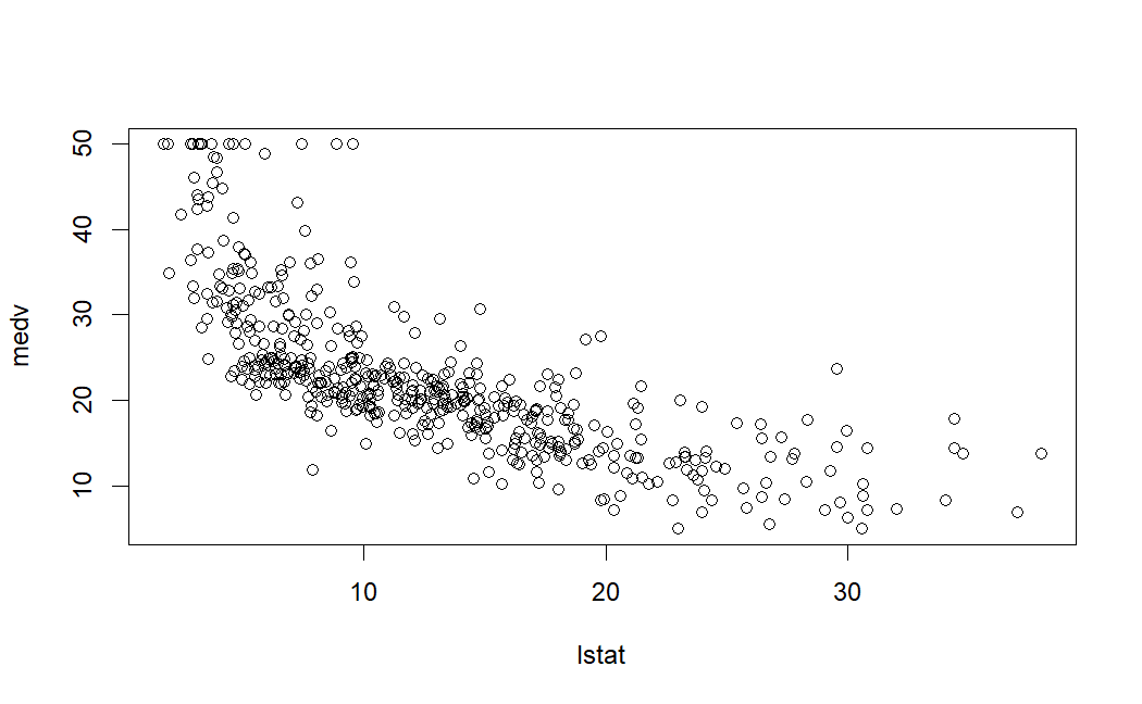
../../_images/mdev_lstat_boston.png — Fig. 42 Plot of mdev vs. lstat from Boston dataset from the R MASS library.#

There does seem to a be linear trend, and we could fit a linear model, which can be represented as be a straight line that ‘’best’’ describes this dataset.

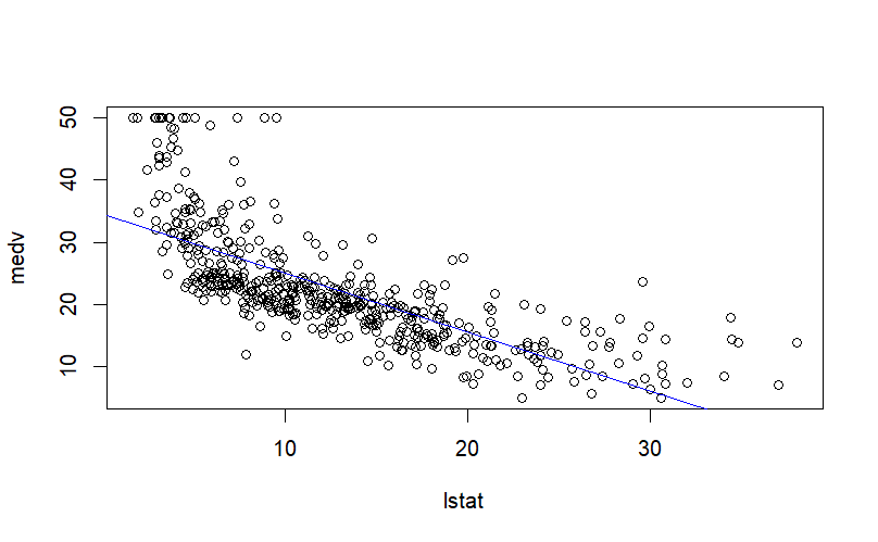
../../_images/mdev_lstat_boston_fitted.png — Fig. 43 A fitted linear model overlaying the data-points from the figure above.#

Let’s get more formal. In a simple linear model, for each value $x$ of the predictor, the response is a random variable denoted by $Y|x$. The model takes the following form:

\[\begin{align*} E[Y|x] &= \beta_{0} + \beta_{1} x \\ Var (Y|x) &= {\sigma}^2. \end{align*}\]

Parameter estimation#

The parameters $\beta_{0}$, $\beta_{1}$, $\sigma$ are estimated from data.

Let $(x_1,y_1), (x_2,y_2), \ldots, (x_n,y_n)$ be $n$ observations, where the $x$ and $y$ values are instances of the predictor and response variables, respectively.

One way to estimate $\beta_{0}$ and $\beta_{1}$ is the so-called least-squares estimation, in which we try to minimize the sum of the residuals. A residual, $e_i$ for the $i$-th observation is the difference between $y_i$ and its value predicted by the model and is given by:

\[e_i = y_i - \beta_{0} - \beta_{1}x_i.\]

The sum of the residuals, $RSS$ is defined as:

\[RSS(\beta_{0},\beta_{1}) = \sum\limits_{i=1}^{n} {e_i}^2.\]

Applying some basic calculus, we can show that $\hat{\beta_{0}}$ and $\hat{\beta_{1}}$ that minimize $RSS$ are:

\[\begin{align*} \hat{\beta_{1}} &= \frac{\sum_{i=1}^{n} (x_i- \bar{x})(y_i- \bar{y})}{\sum_{i=1}^{n} (x_i- \bar{x})^2},\\ \hat{\beta_{0}} &= \bar{y} - \hat{\beta_{1}}\bar{x},\\ \end{align*}\]

where $\bar{x}$ and $\bar{y}$ are the sample means.

The estimator of the variance $\sigma^2$ is:

\[s^2 = \frac{RSS}{n-2}.\]

Estimating the standard errors#

Assuming that there exist true $\beta_{0}$,$\beta_{1}$, we wish to estimate how accurate the $\hat{\beta_{0}}$ and $\hat{\beta_{1}}$ estimates are. For this we calculate the standard error, $SE$ of the estimated coefficients, given by:

\[SE(\hat{\beta_{0}})^2 = \sigma^2 \left(\frac{1}{n} + \frac{{\bar{x}}^2}{\sum_{i=1}^{n} (x_i- \bar{x})^2} \right),\]

and

\[SE(\hat{\beta_{1}})^2 = \frac{\sigma^2}{\sum_{i=1}^{n} (x_i- \bar{x})^2}.\]

To get an estimate of the standard error, the variance $\sigma^2$ is replaced by its estimate $s^2$.

The standard errors are needed for computing confidence intervals and hypothesis tests on the coefficients. Let’s look at the latter.

Testing for relationship between response and predictor#

In many cases, we don’t really use the model to predict what values of $Y|x$ we expect given a certain $x$, but rather we wish to test the (null) hypothesis that there is no relationship between the response and predictor, i.e. $\beta_{1} = 0$.

If we assume that $Y|x$ has a normal distribution, then $\hat{\beta_{1}}$ is also normally distributed. Then we can use the t-statistic:

\[T = \frac{ \hat{\beta_{1}}-0 } { SE(\hat{\beta_{1}}) },\]

as test statistic to compute the significance. Under the null hypothesis ( $\beta_{1} = 0$), $T$ has a t-distribution with $n-2$ degrees of freedom.

Example#

Here is an example of fitting a linear model on the Boston dataset introduced above, setting mdev as the response variable and lstat as the predictor.

library(MASS)
lm.fit <- lm(medv~lstat, data=Boston)
summary(lm.fit)

The output looks like:

Call:
lm(formula = medv ~ lstat, data = Boston)

Residuals:
    Min      1Q  Median      3Q     Max 
-15.168  -3.990  -1.318   2.034  24.500 

Coefficients:
            Estimate Std. Error t value Pr(>|t|)    
(Intercept) 34.55384    0.56263   61.41   <2e-16 ***
lstat       -0.95005    0.03873  -24.53   <2e-16 ***
---
Signif. codes:  0 ‘***’ 0.001 ‘**’ 0.01 ‘*’ 0.05 ‘.’ 0.1 ‘ ’ 1

Residual standard error: 6.216 on 504 degrees of freedom
Multiple R-squared:  0.5441,	Adjusted R-squared:  0.5432 
F-statistic: 601.6 on 1 and 504 DF,  p-value: < 2.2e-16

In this example, Intercept corresponds to ${\beta}_0$ and lstat refers to ${\beta}_1$. We see that they have been estimated to be 34.55384 and -0.95005, respectively; and that we can safely reject the null hypothesis that lstat and mdev are not related. In this case, this is actually quite evident from the plot in Fig. 43, with the blue line is the line $mdev = 34.55384 -0.95005 \times lstat$.

Categorical/Qualitative Predictor#

In many cases, the predictor might be a categorical variable, also called a factor, as opposed to a covariate when its a continuous variable. Take for example the Credit Card Balance Data provided in the ISLR R package. From this dataset, let’s take Balance as the response variable and Gender as the factor. The former is the average credit card balance and the latter is the gender of an individual. The data looks like this:

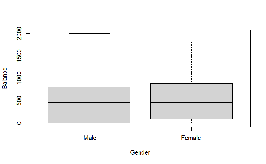
../../_images/balance_gender_credit.png — Fig. 44 Plot of balance vs. gender from the Credit dataset from the R ISLR library.#

Although there doesn’t seem to a visually evident linear relationship, let’s go ahead and set up a linear model. The predictor $x$ can be defined as a binary indicator variable that represents Female by 1 and Male by 0. The response variable $Y$ represents the credit card balance. The linear model takes the same form as before.

\[\begin{align*} E[Y|x] &= \beta_{0} + \beta_{1} x \\ Var (Y|x) &= {\sigma}^2. \end{align*}\]

The coefficients now have an easier interpretation: $\beta_{0}$ is the mean of the balance of males, and $\beta_{0}+\beta_{1}$ is the mean of females.

All the theory discussed above for the covariates hold just as well for factors as well. Here is the result of linear model fitting in R:

Call:
lm(formula = Balance ~ Gender, data = Credit)

Residuals:
    Min      1Q  Median      3Q     Max 
-529.54 -455.35  -60.17  334.71 1489.20 

Coefficients:
             Estimate Std. Error t value Pr(>|t|)    
(Intercept)    509.80      33.13  15.389   <2e-16 ***
GenderFemale    19.73      46.05   0.429    0.669    
---
Signif. codes:  0 ‘***’ 0.001 ‘**’ 0.01 ‘*’ 0.05 ‘.’ 0.1 ‘ ’ 1

Residual standard error: 460.2 on 398 degrees of freedom
Multiple R-squared:  0.0004611,	Adjusted R-squared:  -0.00205 
F-statistic: 0.1836 on 1 and 398 DF,  p-value: 0.6685

As you might have suspected, the p-value for $\beta_{1}$ is high, suggesting that the difference in credit card balance between males and females is not significant.

In fact, it is quite often the case in bioinformatics that the predictor is categorical. For example in the next section we will see how to model differences in gene expression between sample groups, e.g. treated with some drugs vs. untreated.

Extensions#

Multiple covariates
Multiple factors and choice of encodings
Model accuracy
Regularization
Generalized linear models

Spherical cow#

In the simple linear model described above, we assumed that $Y|x$ follows a normal distribution and that the variance is the same $\sigma^2$ for all $Y|x$. These assumptions need to hold true for reliable testing and confidence interval computations. But almost always they are violated, just like the physicist’s assumption of a cow being perfectly spherical.

There are several ways to deal with the problem of non-normality and unequal variances. The prominent ones include:

transformation (e.g. log or square-root) of the response variable and
weighting the observation by their precision.

We will visit these ideas in the context of comparing gene expression.

References#

Chapter 3 of James, Witten, Hasite, Tibshirani: An Introduction to Statistical Learning with Applications in R (2017), Springer Texts in Statistics.
Dunn, Smyth: Generalized Linear Models With Examples in R (2018), Springer.