Local alignment

Local alignment#

Use cases:#

Searching a protein database with a query sequence
Comparing human and mouse genomes to find regions of local similarity, etc.
Aligning DNA sequencing reads from high-throughput sequencers to reference sequences

Scoring a local alignment#

We will use the same scoring scheme as we did with global alignment, except that we want only parts of the sequences that are homologous to contribute to the score (e.g. the green segments below).

../../_images/local_alignment.svg — Fig. 27 Local alignment scoring#

Smith-Waterman algorithm for local alignment#

Like the global alignment problem, the problem of finding a highest-scoring local alignment can also be solved by dynamic programming.

Let $A$ and $B$ be the two input sequences of lengths $m$ and $n$ respectively; let $A[i]$ be the $i$-th residue of sequence $A$ and $A[i:j]$ be the substring $A[i], A[i+1],\ldots, A[j]$. Let $M=[m_{xy}]$ be the substitution matrix. For simplicity, let’s assume linear gap penalty of $g$ for now.

We have to be a bit more clever with defining subproblems here, since an optimal local alignment between $A[1:i]$ and $B[1:j]$ don’t necessarily involve $A[i]$ or $B[j]$.

Instead, define $S_{ij}$ to be the score of a highest scoring global alignment among global alignments of suffixes of $A[1:i]$ and $B[1:j]$. That is, let $SA_i$ and $SB_j$ be the set of all suffixes (include the empty string) of $A[1:i]$ and $B[1:j]$, respectively. Then

\[\begin{split}S_{ij} = \max_{\substack{X \in SA_i \\ Y \in SB_i}} \left( \text{score of global alignment between $X$ and $Y$} \right)\end{split}\]

Given this definition of $S_{ij}$, the following recurrence relation can be derived:

\[\begin{split}\begin{align} S_{ij} &= \max \begin{cases} S_{i-1,j-1} + m_{A[i],B[j]}\\ S_{i-1,j} + g\\ S_{i,j-1} + g \\ 0 \\ \end{cases} \\[2em] S_{0,j} &= 0 \text{ for } 0 \leq j \leq n \\ S_{i,0} &= 0 \text{ for } 0 \leq i \leq m \end{align}\end{split}\]

The first 3 cases of the recurrence relation above follow from the same reasoning as with the global alignment recurrence. The last one pertains to the case in which the highest scoring global alignment is between the empty suffixes.

The optimal local alignment score is then the maximum of $S_{ij}$ over all possible $i,j$ pairs. As with global alignment dynamic programming, $S_{ij}$ can be computed bottom-up; and to obtain the alignment itself, we need to perform traceback from a cell that has highest $S_{ij}$ to a cell where it is 0.

Here is an online demonstration.

For affine gap penalty, we need to have extra variables that keep track of whether we are opening a gap or extending a gap.

Time complexity#

There are $\Theta(mn)$ cells to compute and each cell takes $\Theta(1)$ time to compute. So the running time is $\Theta(mn)$. Even though the search space is much larger than global alignment, interestingly the running time is the same as that of global alignment.

Given the size of sequence data we deal with these days, quadratic time complexity is just not ok. Imagine trying to search for a query protein sequence containing 100 amino acids against the the UniProt database. The current release has over 250 million entries with a total of more than 90 billion amino acids. How many cells does the dynamic programming algorithm need to compute? With a great CPU and highly optimized computer program, you might be able to compute roughly 1 billion cells per second. How long will it take to compute all the cells?

Heuristics for faster local alignments#

The most popular local alignment tool for database is BLAST. There is a web interface here. Just for fun, try searching a segment of the human ACE2 sequence from your assignment before.

hayvraklmnaypsyispigclpahllgdmwgrfwtnlysltvpfgqkpnidvtdamvdq

How is it that BLAST does not take forever to find local alignments of this sequence to other entries in the database?

Seed and extend#

All modern local aligners designed to be used for large datasets rely on the idea of seed-and-extend. The idea is that sequence segments that would achieve a high local alignment score are likely to contain short exact matches called seeds. A seed is then extended to a longer alignment by dynamic programming in the region at the two ends of the seeds. Not all seeds will lead to a high-scoring local alignment, so an extension is discontinued if the score drops below a certain threshold.

How to find seeds quickly?#

For seed-and-extend to work, we need to be able to find seeds quickly. This can be done by first building an index of the reference sequence(s). Then seeds can be identified by searching substrings of query on this index.

One popular indexing data-structures is a suffix array. A suffix array contains the indexes of the lexicographically sorted suffixes of a string. The following is an example.

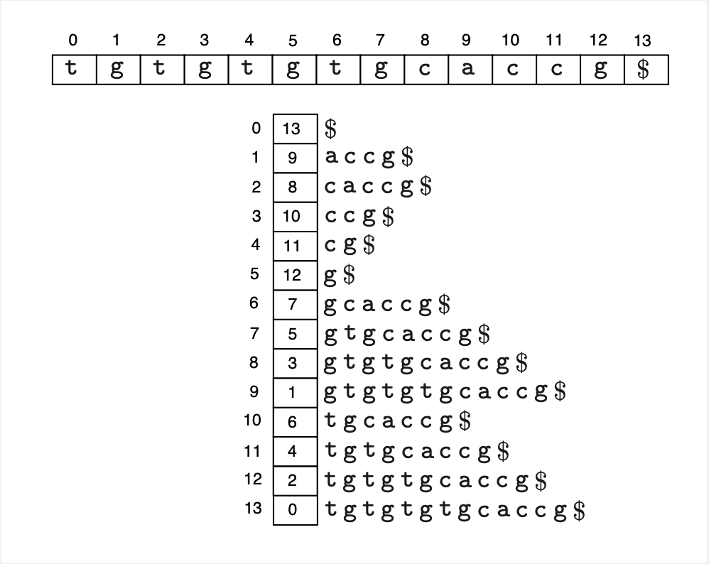
../../_images/suffix_array_example.jpg — Fig. 29 A suffix array(below) of a string (above).#

Given a string of size $n$, its suffix array can be constructed in $\Theta(n)$ time. If we represent an integer by 4 bytes, then the suffix array will take $4n$ bytes to store. Finding whether a certain query substring of size $q$ is present in the string can be done by binary search on the suffix array in $O(q \log n)$ time.

Improvements to suffix array.

Variations to exact seeds#

spaced seed
subset seed

Statistical significance of local alignments#

Suppose you found a highest scoring local alignment of score $s$ between two sequences $A$ and $B$ of lengths $m$ and $n$ respectively. Is this alignment an evidence of true homology or could it have been obtained just by chance? That is, we wish to compute the probability that two unrelated sequences of the same lengths would achieve a score higher than $s$.

First off, how do we define unrelated-ness? A mathematically convenient way is to think of two random sequences, each generated from a given background frequency of nucleotides (or amino acids for protein sequences). Let $S$ be a random variable representing the optimal local alignment score of two random sequences of lengths $m$ and $n$.

What is the probability distribution of $S$? Could we approximate it with a normal distribution so that we can easily compute $p(S \geq s)$ through e.g. z-scores? It turns out not. For the case of ungapped local alignments, it can be shown analytically that $S$ follows a so-called extreme value distribution (aka Gumbel distribution). The derivation is quite complicated, but the idea is as follows. First, under assumptions that $m$ and $n$ are sufficiently large, the number of distinct local alignments with scores at least $s$ can approximated by a Poisson distribution with expectation:

\[E[\text{no. of alignments with score } S \geq s] = kmne^{-\lambda s},\]

where the two parameters $k$ and $\lambda$ are estimated from the background frequencies and the scoring scheme. Then it follows that $p(S \geq s)$ which is the probability that there is at least 1 local alignment with score higher than $s$ is:

\[p(S \geq s) = 1 - e^{-kmne^{-\lambda s}}.\]

The E-value shown above is used rather than the probability, since it’s easier to interpret. And anyway, for small values, E-value is very close to p-value, since for a real number $x$, $e^x \approx 1 + x$ when $|x|$ is small.

In the case of database search, a query sequence of length $m$ is compared to many sequences of varying lengths. One easy workaround is to think of the entire database as one long sequence of length $n$. The screenshot below shows a BLAST database search result sorted by E-value.

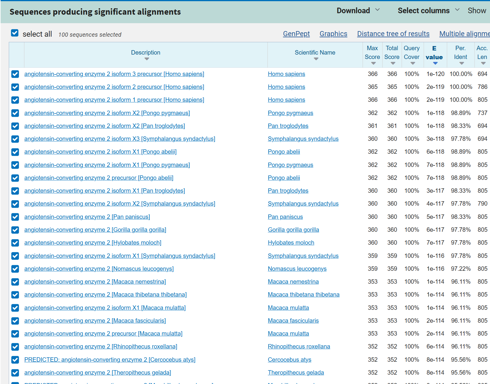
../../_images/BLAST_Evalue.png — Fig. 30 Screenshot of BLAST report.#

Unfortunately, there is no theory for the case of gapped alignment scores. Luckily, empirical evidence suggest that it is ok to assume extreme value distribution for gapped cases. However, the parameters $k$ and $\lambda$ have to be obtained through simulations.

TODO: Edge correction

References#

https://www.ncbi.nlm.nih.gov/BLAST/tutorial/Altschul-1.html