Comparing gene expression levels measured by RNA-seq

Many biological studies revolve around the question of whether or not some genes change their expression levels under different conditions. Different conditions could mean for example when a system undergoes heat stress, or tissues at different stages of (embryonic) development, or normal vs. cancer tissues, etc.

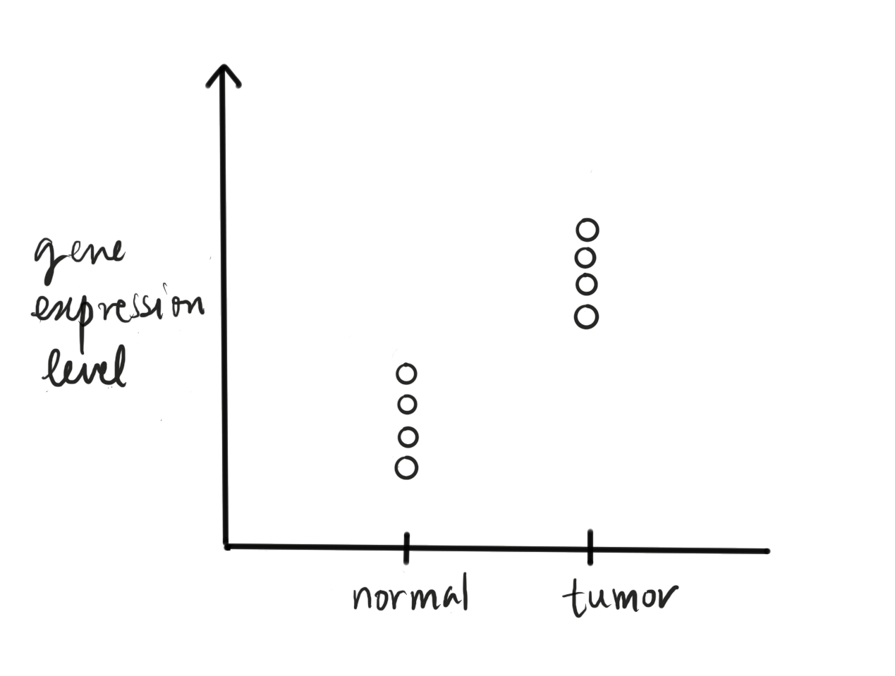
Fig. 46 A typical study design where gene expression is compared across case and control samples..

There are many traditional lab techniques to quantitate gene expression, which is the abundance of mature RNA transcribed from a gene (e.g. variants of PCR, microarray). Here we will focus on a relatively new technology called RNA-seq, which utilizes modern sequencers to sequence all RNA molecules present in the specimen.

RNA-seq and the data-generation process

The typical data generation process of RNA-seq goes as follows (see figure below). From a biological sample, mature RNAis extracted. Ribosomal RNA (rRNA) make up a vast majority (80-90%) of RNA in a cell, and it is excluded them from extraction by selectively degrading them or selectively extract only RNAs with a poly-A tail while rRNAs don’t have such tails. This can be used as signatures to selective extraction. There are also techniques to selectively degrade rRNA. Next, the RNA molecules are fragmented, and double-stranded cDNA molecules are synthesized from the RNA fragments. The cDNA are sequenced using a high-throughput sequencer, resulting in a huge sequence dataset.

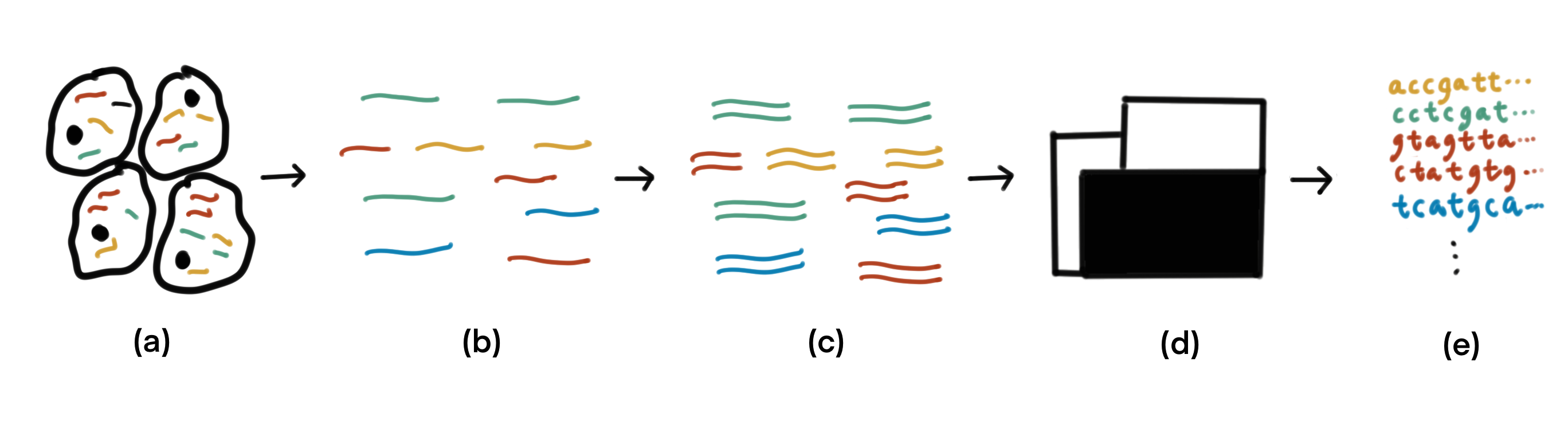
Fig. 47 Given a biological sample (a), mature RNA is extracted and fragmented (b). (c) Double-stranded cDNA molecules are synthesized from the RNA fragments. The cDNA are fed to a sequencer (d) to obtain sequence data (e).

Read counts as proxy for gene expression level

The sequence are read-outs of fragments of mature RNA. They can be used in many ways, but the one we will be interested in here is in measuring gene expression, which here means the number of RNA molecules transcribed from a gene.

For this, we find pairwise alignments of each sequence to a database of known transcript sequences (Fig. 48). The number of sequences aligning to a certain transcript is used as a measure of the number of copies of the transcript present in the sample. Suppose the database contains the sequence of a dominant transcript isoform for each gene of the species under study, then the counts give a relative measure of gene expression of all the genes.

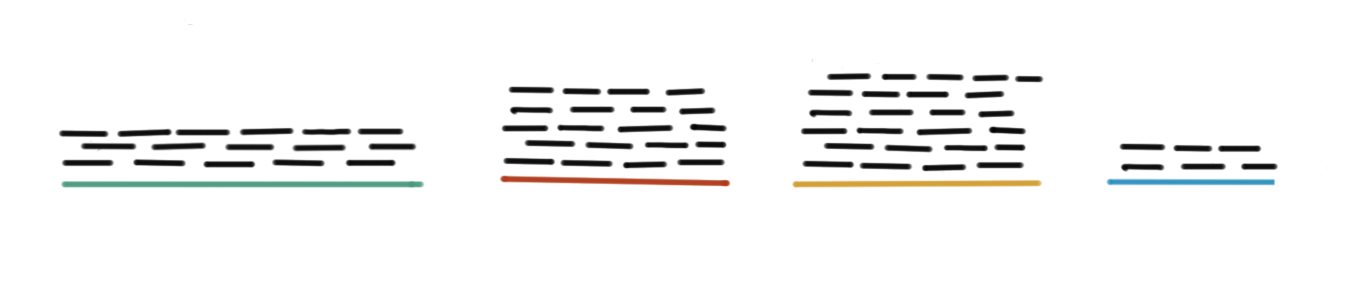
Fig. 48 Measuring gene expression. RNA-seq reads (represented by black short lines) are aligned to a reference database containing transcript sequences (represented by colored lines). The number of reads aligning to each transcript is used as a proxy.

Note that a longer transcript will have more reads mapped to it than a shorter one, even if both are equally abundant in the sample. If the goal is to compare between different genes in a sample, then we need to normalize by length. But here, we will be comparing the same gene under two conditions, so normalizing by length is not necessary. What is necessary though is normalizing by the overall number of reads generated when sequencing a sample (a.k.a sequencing depth).

Some pertinent details have been omitted in the description above. Since we interested in just the counts, then it suffices to identify which gene each read maps to, and an alignment itself is an overkill. There are methods (see e.g. here) to compute the mappings without fully computing alignments. Also, because genomes contain many repeat elements, reads might map to multiple genes, in which case a meaningful disambiguation scheme is required (see e.g. here).

Modeling RNA-seq data

Linear model for one gene

RNA-seq can measure the expression of all genes at once, but in a typical analysis workflow, we build a separate model for each gene. Consider the simple case where there are two conditions, say disease vs. normal. This can be represented by a binary predictor variable \(x\), with normal encoded as 0 and disease as 1. Let \(Y|x\) be the random variable representing number of reads, normalized by sequencing depth, mapping to the gene gene for a particular value of \(x\). Following our earlier discussion, we could define a linear model as:

\[\begin{align*} E[Y|x] &= \beta_{0} + \beta_{1} x \\ Var (Y|x) &= {\sigma}^2. \end{align*}\]

After estimating \(\beta_{0}\), \(\beta_{1}\), and var (Y|x), and their standard errors, from observed expression data, we could test the null hypothesis that the gene \(g\) is not differentially expressed by testing the null hypothesis that \(\beta_{1}=0\).

However, this model violates some of the assumptions of the simple linear model which are needed for reliable hypothesis testing and confidence interval computation. First, \(Y|x\) represents discrete counts and is not described by a normal distribution. Next \(Y|x\) do not all have equal variances. It is typical for random variables representing counts to have a mean-variance relation in which the larger the mean, larger the variance. Another reason for unequal variances could be that disease samples exhibit more variability than normal ones.

Dealing with unequal variances and non-normality

One technique to deal with unequal variances and non-normal distribution is data transformation. The idea is to log-transform the response variable, and fit a linear model on the transformed data. In the case of RNA-seq, we define \(Y_{x}\) in the model to represent the log of read counts (instead of raw counts) normalized by sequencing depth.

More formally, let \(r_{gi}\) be the number of reads mapped to gene \(g\) in the \(i\)-th sample. And let \(R_i\) be the total number of mapped reads:

\[R_{i} = \sum\limits_{g} r_{gi}\]

Then log-counts per million are defined as:

\[y_{gi} = \log_2 \left( \frac{r_{gi}+0.5}{R_i + 1.0} \times 10^6 \right).\]

The offset of 0.5 in the numerator prevents log of zero, and the offset of 1 in the denominator ensures the ratio is between 0 and 1. The \(y_{gi}\) will serve as an instance of the response variable.

Another way to deal with unequal variance is to weigh the observations based on their precision.

Here is a paper describing applying these ideas (and more).

Generalized linear model

Yet another option for modeling RNA-seq data is to do away with any assumption of normality and to explicitly model the counts data by a model appropriate for it, like the negative binomial distribution.

Briefly, let \(Y|x\) be the random variable representing the number of reads mapped to the gene under consideration for condition \(x\), normalized by sequencing depth. We assume that the distribution of \(Y|x\) is a negative binomial with a mean \(\mu_{x}\) and dispersion \(\alpha_{x}\). And the model looks like:

\[\begin{align*} Y|x &\sim NB(\mu_{x},\alpha_{x}) \\ \log_{2} \mu_{gx} &= \beta_{0} + \beta_{1} x \end{align*}\]

Parameter estimation for this kind of model is done by maximum likelihood estimation. Testing the hypothesis \(\beta_{1}=0\), that there is no differential expression, can be done by a Wald test. Here is a paper describing applying these ideas (and more).

Multiple testing correction

The model fitting and inference procedure is done for each of the thousands of genes that is measured by RNA-seq. Even if none of the genes were differentially expressed, some of the p-values might be lower than the threshold you set for significance, just by chance. This problem of false-positives creeping in because you conducted many hypothesis tests is called multiple testing or multiple comparison problem. This problem is serious especially with RNA-seq in which we can measure >15000 genes at the same time and conduct that many hypothesis tests simultaneously.

To get a feel for the seriousness, let’s look at some numbers. Suppose you decide to reject the null hypothesis (that a gene is not differentially expressed) when the p-value falls below \(\alpha = 0.05\). That is, under the null hypothesis, the probability of a false positive is 0.05. Now suppose you test for differential expression on 20 genes, and assume that none are differentially expressed. The probability of least one false positive is:

\[\begin{split}\begin{align*} p(\text{ 1 or more significant result}) &= 1 - p(\text{no significant result}) \\ &= 1 - (1-0.05)^{20} \\ &= 0.64. \end{align*}\end{split}\]

This error rate has a fancy name: family-wise error rate. If the number of genes was 100, the probability of at least one false positive becomes 0.994. This issue is severe already at 100, forget about testing >15000 without getting flooded by false positives.

Methods to deal with multiple testing adjusts the p-value or the threshold to account for the multiple tests.

Controlling family-wise error rate

A straightforward method is to use a stricter significance threshold, from \(\alpha\) to \(\alpha/\text{no. of tests}\). So for the example above with 20 tests, we set the significance threshold from \(0.05\) to \(0.05/20 = 0.0025\). And the probability of at least 1 false positive now drops to:

\[\begin{split}\begin{align*} p(\text{ 1 or more significant result}) &= 1 - p(\text{no significant result}) \\ &= 1 - (1-0.0025)^{20} \\ &= 0.0488, \end{align*}\end{split}\]

which is what we wanted in the first place.

In reality, not all the null hypotheses tested are true. While controlling the family-wise error rate provides guarantee against false positives; it increases the chance of false negatives (cases where genes are truly differentially expressed, but we decided that they are not). This is maybe fine for some settings, but with high-throughput techniques like RNA-seq, we usually aim to generate new hypotheses that can be further validated by more experiments. With the stringent Bonferroni correction, we risk losing out on making some wonderful discoveries.

Controlling false discovery rate

Another way to deal with the multiple testing is to control false discovery rate (FDR), which is the rate that significant results are truly null. For example, a FDR of 5% would mean that if we found 100 genes to statistically significantly differentially expressed, 5 of them on average are false positives. The Benjamini-Hochberg procedure achieves this by doing the following.

Let \(H_1, H_2, \ldots, H_m\) be the hypotheses being tested.
Let \(p_1, p_2, \ldots , p_m\) be the corresponding p-values.
Let \(q^*\) be the user-set FDR.

Steps:

1. Sort the p-values in non-increasing order: \(p_{(1)} \leq p_{(2)}\leq \cdots \leq p_{(m)}\).

2. Let \(k\) be the largest index \(i\) such that \(p_{(i)} \leq \frac{i}{m}q*\).

3. Reject the corresponding hypotheses \(H_{(1)}, H_{(2)}, \ldots, H_{(k)}\).

Here is another method for multiple testing correction, which claims to be more suitable for genome-wide studies, like RNA-seq, that generate thousands of hypotheses.

References

• Chapter 4 of Dunn, Smyth: Generalized Linear Models With Examples in R (2018), Springer.

• voom: precision weights unlock linear model analysis tools for RNA-seq read counts

• Statistical significance for genome-wide studies https://doi.org/10.1073/pnas.1530509100

• Benjamini Y, Hochberg Y. Controlling the false discovery rate: a practical and powerful approach to multiple testing. Journal of the Royal Statistical Society. Series B (Methodological) 1995:289–300

• https://doi.org/10.1038/s41576-019-0150-2